Routing Algorithms¶

LEOPath exposes routing algorithms through a pluggable interface. Each one computes forwarding state for ground-station-to-ground-station traffic across the satellite network, and every algorithm sees the same topology snapshots, so runs are directly comparable.

Implemented algorithms¶

• shortest_path_link_state: Dijkstra over the dynamic ISL graph, recomputed from scratch at every snapshot.
• topological_routing: 6G-RUPA addressing with neighbor-based forwarding, where the forwarding decision comes from the distance between the current node's address and the destination's.
• dra_routing: the DRA family of Ekici, Akyildiz and Bender, restricted to hop-count distance on logical (plane, slot) coordinates.
• explicit_path_routing: a protocol-agnostic proxy for centrally planned explicit paths, with the path pinned across one or more snapshots.

dra_routing and topological_routing share the same forwarding machinery and differ only in the distance function, which is deliberate: a run of one against the other isolates the contribution of the distance metric with everything else held fixed. dra_routing overrides any distance_mode you pass so a run cannot quietly turn into the weighted variant.

Assumptions and limitations¶

• Every algorithm attaches ground stations to the nearest visible satellite.
• explicit_path_routing plans on the current snapshot. Planning against a predicted future snapshot is deliberately left out.
• Topological addressing assumes plane and satellite indices stay stable, which is what makes the address meaningful as a location.
• ISL failures are not modelled unless you inject them.
• Inter-satellite links are built as a +Grid, four terminals per satellite. Starlink flies three lasers, and ISL Topology works out what that layout would do to the pivot estimator. It isn't built yet.

Design considerations¶

Shortest-path link-state¶

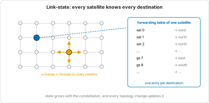
Full topology knowledge at every snapshot, so it gives the lower bound on stretch and path length that everything else is measured against. It also sets the ceiling on forwarding state, since each satellite ends up holding an entry per destination.

Topological routing¶

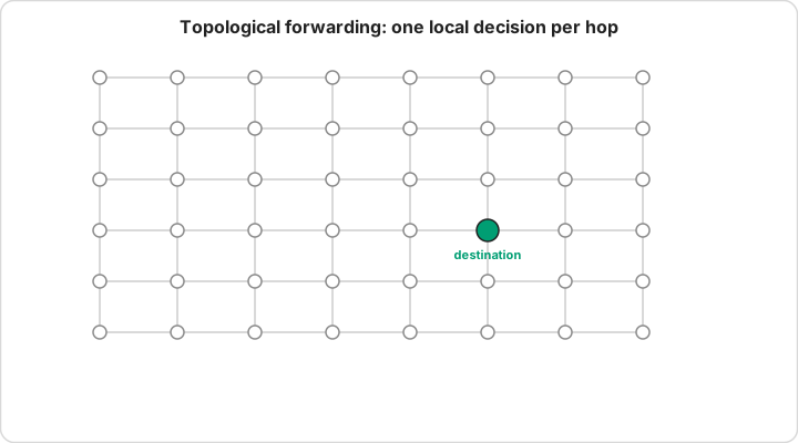
Structured addressing replaces full topology state. A satellite decides the next hop from the topological distance between its neighbors' addresses and the destination address, which means state scales with node degree rather than constellation size. The trade the design makes is low, stable state against strict path optimality; whether it actually costs any optimality depends on the distance metric.

The distance_mode parameter selects that metric:

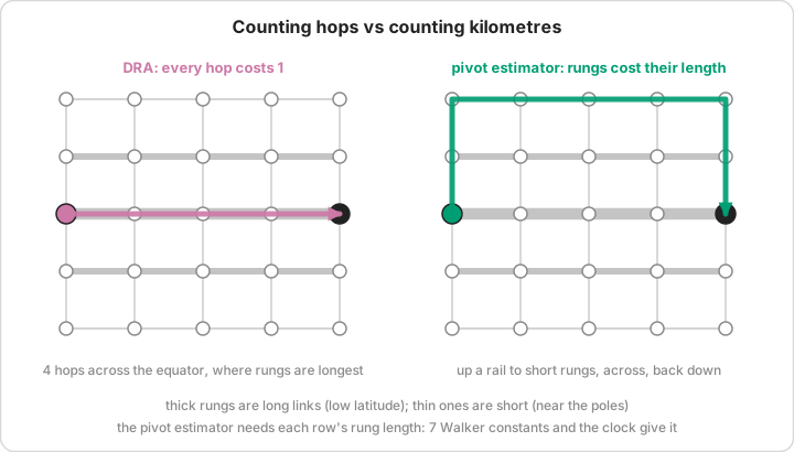
• torus_unit: hop count on the logical torus. Every edge costs 1, so the estimator is blind to how much physically longer an inter-plane ISL is near the equator than near the poles. This is what dra_routing pins.
• torus_weighted_lookahead (the default): weighted progress with a one-hop lookahead.
• torus_weighted_pivot: builds a per-snapshot weight model from ISL lengths, then estimates distance through row and column pivots. This is the mode the Computer Networks paper evaluates.

Where the geometry comes from¶

A satellite can range its own links and nothing else. To rank its neighbours it still needs every other ISL length in the shell, and geometry_source decides where those come from:

  observed    the snapshot as routed, failures included    every satellite knows every failure: not realistic
  nominal     the failure-free graph, SGP4-measured        every length measured, would have to be flooded
  derived     the failure-free wiring, lengths computed    7 constants and the clock, nothing flooded
              from the shell's Walker constants

derived is the one that matches the design. leopath/topology/walker_geometry.py holds a shell as its constants (planes, satellites per plane, inclination, mean motion, how far the nodes are spread, the half-slot phasing of odd planes, the epoch) and carries every satellite forward on a circular orbit with SGP4's own secular rates. Those rates come from SGP4's initialisation, which is itself a closed-form function of the same constants, so a satellite can compute them once when it joins the layer. Against SGP4 on the four built-in shells the derived lengths are off by 0.05-0.09% on rails and at most 0.26% on rungs (1% on one short Kuiper rung, 1.6 km of 154), with about 10 km of position error left over from SGP4's periodic terms.

That turns the pivot tables into a cache. Every rail of a circular shell has one length, and a rung's length depends only on its row, the parity of its plane and the time, so DerivedPivotEstimator in topological_routing/derived_pivot.py answers a pivot query in O(S) from the constants alone. tests/forwarding_state/topological_routing/test_derived_pivot.py checks it against the tabled estimator on every satellite pair of four shell shapes, delta, odd plane count, star and unphased, at three times, and they agree to 1e-9. The simulator still builds the tables because they're faster to query; nothing it reports depends on them being there. Per snapshot it records aux_geometry_required_entries, what the estimator needs a satellite to hold: 7 under derived, one length per rail and rung otherwise.

Measured and derived geometry route the same way. Over 1 536 paired runs, four constellations and every failure condition, switching changed delivery of the full scheme by nothing and of the plain rule by at most 0.00044, and distance stretch by at most 0.0033.

The pivot estimator also needs to know how the shell is wired, which the harness passes as isl_wiring: plus_grid, or brick_a / brick_b for the three-terminal layouts of ISL Topology, where no single row carries a crossing and the estimator prices a closed-form staircase instead.

Parameter notes:

• plane_weight, sat_weight, shell_weight: relative costs used by the weighted modes.
• gs_addressing: attachment makes a ground station's address name the satellite it is attached to; visibility (the default) keeps the address stable and minimises over every visible egress instead.
• gs_attachment_count: under attachment addressing, advertise the K nearest assigned satellite addresses (default 1).
• gs_attachment_policy: independent gives every station its unconstrained top-K set, so one satellite can serve many stations, as real satellites do; exclusive solves a minimum-cost assignment in which each satellite serves at most one ground station, a deliberately pessimistic case.
• gs_address_policy: with K above 1, which of a station's K addresses its flows use. sticky_nearest (the default), nearest, requester_aware or per_flow_pair; see A station with several attachments.
• gs_attachment_order: which visible satellites a station attaches to first. nearest (the default), nearest_ascending or one_per_half; see Two halves of a shell.

Where the destination address comes from¶

A packet carries the destination's 6G-RUPA address, and gs_addressing decides what that address means for a ground station.

  ATTACHMENT                              VISIBILITY (the default)

  address names the satellite the         address is stable and says nothing
  station is attached to:                 about location:
     (shell 0, plane 3, slot 1, x=2)         "ground station 7"

  a satellite reads plane 3, slot 1       a satellite works out which
  and forwards that way. Done.            satellites can see station 7,
                                          then minimises over all of them

  needs: nothing about the station        needs: the station's coordinates,
                                          on board, plus a visibility
                                          calculation every snapshot

  evaluates 1 distance per decision       evaluates ~16, one per visible
                                          egress

Attachment is what the addressing scheme describes, and it's the cheaper of the two by some distance: a forwarding satellite holds no ground-station table and does no visibility arithmetic. The station attaches to its nearest live visible satellite, which is the rule _detect_gsl_changes already applied to decide when an address has to change, so nothing new decides it.

What it costs is renumbering. A satellite stays above a fixed point for a few minutes, so the address follows it and then has to change:

  t = 0                    t = 5 min                t = 10 min

     e1 = (p3,s1)             e2 = (p3,s2)             e3 = (p4,s2)
      |                        |                        |
     ~~~~                     ~~~~                     ~~~~
       g                        g                        g

  address (0,3,1,2)        address (0,3,2,2)        address (0,4,2,2)
  name    "madrid-gw-3"    unchanged                unchanged

Each change costs a directory update and a flow update to the far end of every active flow; aux_gs_renumberings counts the stations whose advertised addresses changed in a snapshot. Connections survive it, since EFCP keys on port-ids rather than addresses.

A station with several attachments¶

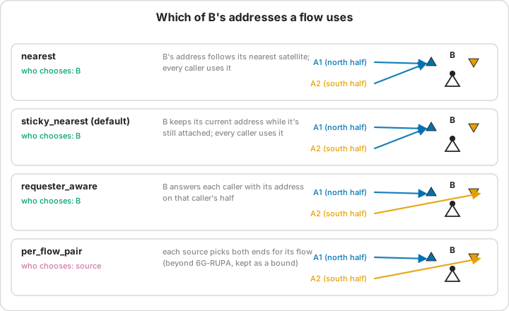
Set gs_attachment_count above 1 and a station is attached to K satellites at once, holding one address under each. Its IPC process accepts packets sent to any of them, the way a 6G-RUPA IPC process accepts any of its synonyms. A packet still carries exactly one destination address, though, and no satellite along the way may swap it for another of the station's addresses, so something has to decide which of the K a flow uses. That decision is a policy, gs_address_policy:

  station g, K = 2                     sticky_nearest (the default)

    e1 = (p3,s1)     e2 = (p3,s2)      g's current address sits under e1;
     |                |                the one under e2 is a standby that
    ~~~~             ~~~~              is already live
        \          /
            g                          e1 drifts off but stays one of g's
                                       two attachments: keep it, no cost

                                       e1 drops out of the pair: g moves to
                                       its nearest remaining attachment and
                                       every flow of g moves with it

The directory hands out a station's current address, so under the first two policies link-state and topological routing route to the same pair of satellites and differ only in how they forward. Under sticky_nearest a second attachment buys fewer renumberings, plus a standby address that is already live when the current one goes, which lets a station renumber make-before-break. It doesn't buy a shorter path; if anything the current address drifts away from the nearest satellite until it has to move. Only per_flow_pair turns extra attachments into route choice, and it gets there by letting a source choose its peer's address flow by flow, which neither 6G-RUPA, the RINA specification it builds on, nor IRATI does. Treat it as a bound.

A station that renumbers sends one flow update to each peer, counted as aux_gs_current_address_changes and aux_flow_update_messages. The simulator counts those messages but doesn't time them, so the window in which the old address still works and the packets in flight across a change sit outside what a snapshot can show.

Two halves of a shell¶

Attaching to the nearest satellite is cheap, and on a Walker delta shell it can send a packet around the planet.

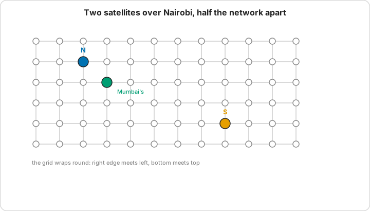
Over any station, satellites cross the sky on two kinds of pass, northbound (ascending) and southbound (descending), and on the logical grid the two kinds sit about half the shell apart:

  Nairobi at t = 0 on Starlink, both satellites 682 km away

  northbound (28, 0)  --  6 275 km from Mumbai's satellite (31, 1)  -> 23 ms
  southbound (64, 11) -- 52 665 km from the same satellite          -> 178 ms

  36 planes and 11 slots apart: half of 72 and half of 22

Link-state pays exactly the same, since the address names the far satellite and forwarding only follows it. Over 24 stations, about three quarters of station pairs have at least one end on the half the best route doesn't use, and those pairs carry 93-95% of the extra delay on Starlink, Kuiper and Telesat (scripts/pass_direction_check.py, scripts/decompose_attachment_cost.py). OneWeb, a Walker star, barely has the problem.

Which half suits a flow depends on both ends, so no rule a station applies alone can always get it right. The cost splits along a line 6G-RUPA already draws. The source end is which satellite A transmits through: A has K ports, and picking the uplink for a destination is ordinary forwarding. The destination end is which of B's addresses the flow carries, and that's settled at flow allocation, where the directory may take the requester's location into account. Two settings follow:

• gs_attachment_order: nearest_ascending prefers northbound satellites. A station can apply it alone and it helps, but for about a third of pairs the best route uses the southbound half at both ends.
• gs_attachment_order: one_per_half with gs_attachment_count: 2 gives every station an address on each half, and gs_address_policy: requester_aware uses it: the directory resolves B to the synonym on the half that suits A, and A uplinks through whichever attachment suits that address. After B's next address change the flow moves to B's current address, as the 6G-RUPA flow allocator prescribes.

Holding an address on each half changes nothing by itself: one_per_half with sticky_nearest costs the same as one attachment, because every flow still uses the current address. The gain comes from the directory choosing per requester.

Failures need no special handling here. apply_failures strips dead satellites from the visibility list before routing runs, so a station whose attachment dies simply attaches to the best survivor at the next snapshot. That is multihoming doing its job, and it is why attachment addressing does not turn every satellite outage into a ground-station outage.

One consequence to keep in mind when reading results: the address fixes the egress, so a satellite cannot route around a poor choice of egress the way it can under visibility. The evaluation reports that cost separately rather than letting it land on the forwarding algorithm; see the stretch factors in Evaluation.

Forwarding under failures¶

Greedy forwarding on a damaged grid can loop. With geometry_source: nominal or derived, a satellite whose best link has failed picks another neighbour, and that neighbour's estimate, which knows nothing about the failure, sends the packet straight back. Three options deal with this, and they stack:

• forwarding_guard: progress forwards only to a neighbour strictly lower in a potential Φ: the estimated distance to the closest satellite that sees the destination, plus that satellite's ground-link length, with ties broken by satellite id. Every hop goes downhill, so a packet can't revisit a satellite, and one with no lower neighbour is at a local minimum, counted in aux_forwarding_exceptions. Φ has to be the same whichever satellite computes it, so only torus_unit and torus_weighted_pivot accept the guard.
• local_repair: square keeps a next hop whose link has failed and reaches it over the shortest live three-hop detour, which on +Grid runs around one grid square. It follows 6G-RUPA's two-step routing, where the path to the next hop is the lower layer's business, and because the decision still names the same next hop the guard's argument holds. A satellite needs the state of links within two hops, nothing more.
• exception_policy: grow adds explicit entries wherever the first two still can't deliver, along the shortest live path, in the style of rule-and-exception forwarding. Entries go only to the satellite where a walk breaks, repeated until every reachable live satellite delivers; aux_exception_entries_one_pass reports the larger placement that gives every failing satellite an entry. It assumes satellites learn failures by flooding only the failures over a topology they already know. Under gs_addressing: attachment a flow keeps its one destination address, so the entries are keyed on the destination satellite rather than the station: (satellite, destination satellite) -> next hop, shared by every flow heading for that address in the snapshot, and the walk restarts after each new entry until it delivers or the destination is cut off.

With all three on, the failure sweep delivered every deliverable pair on all four constellations, and exception state stayed mostly under 1% of link-state's table.

Explicit-path routing¶

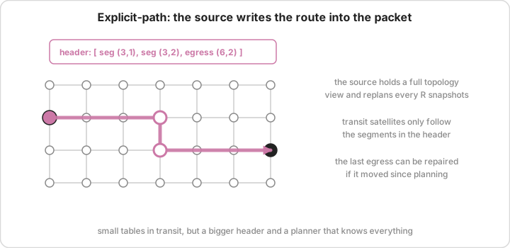
Strict satellite paths are computed per source-satellite / destination-GS pair, either centrally or at the ingress. The packet carries the remaining hop list as a strict SRv6-like adjacency header, so transit satellites only need a local neighbor and interface map. For state accounting, every satellite counts its local neighbor/interface entries, while destination-to-segment ingress bindings are counted only on satellites that currently host a ground-station attachment.

Failover follows SRv6-style local protection rather than a transit shortest-path fallback. When the active adjacency goes away, the intended behaviour is to use a precomputed local backup for that hop; with no backup the packet drops and later packets wait for the ingress or controller to replan. When the planned egress satellite can no longer see the destination ground station, the strict mode drops the packet instead of falling back to a full topology lookup, while the dynamic final-egress mode repairs delivery toward whichever egress is currently visible.

Route plans are exposed for evaluation, adjacency SID lists and strict-header byte counts included. Treat it as a family-level example, not a full SRv6 control plane.

Parameter notes:

• segment_count: affects sampled waypoint metadata only. Strict forwarding follows the adjacency SID list regardless.
• segment_refresh_interval_steps: how many timesteps a strict route plan is reused before replanning. Defaults to 1, which replans every timestep.
• plane_weight, sat_weight and shell_weight are ignored here and are not tuning knobs for this algorithm.

Algorithm parameters¶

Parameters go under simulation.algorithm_params.

Link-state baseline¶

simulation:
  dynamic_state_algorithm: shortest_path_link_state
  algorithm_params:
    gs_addressing: attachment   # optional; default visibility
    gs_attachment_count: 2      # optional; default 1
    gs_attachment_policy: independent
    gs_address_policy: sticky_nearest

• gs_addressing: visibility (the default) lets link-state reach a ground station through any satellite above its horizon. attachment restricts it to the same K assigned satellites used by topological routing, and gs_address_policy then picks the same current addresses for both, so the two differ only in forwarding. exclusive assignment prevents a satellite from being assigned to more than one station.

Topological routing¶

simulation:
  dynamic_state_algorithm: topological_routing
  algorithm_params:
    distance_mode: torus_weighted_pivot
    gs_addressing: attachment
    gs_attachment_count: 2
    gs_attachment_policy: independent
    gs_address_policy: sticky_nearest
    plane_weight: 100.0
    sat_weight: 1.0
    shell_weight: 1000.0

DRA baseline¶

simulation:
  dynamic_state_algorithm: dra_routing

DRA is the topological rule with a hop-count distance (torus_unit), so it accepts every topological option except distance_mode, which it fixes itself: gs_addressing, the attachment options, geometry_source, forwarding_guard, local_repair and exception_policy. Without them it runs as plain DRA. With the same options as topological routing, the two differ only in the distance function, which is the controlled comparison the failure sweep's dra_scheme_* variants make.

Explicit-path routing¶

simulation:
  dynamic_state_algorithm: explicit_path_routing
  algorithm_params:
    segment_count: 2
    segment_refresh_interval_steps: 1

The paper matrix runs all four against the same snapshots, with torus_weighted_pivot as the topological distance mode.

Topological routing with every failure option on:

simulation:
  dynamic_state_algorithm: topological_routing
  algorithm_params:
    distance_mode: torus_weighted_pivot
    geometry_source: derived     # or nominal: same routes, measured lengths
    forwarding_guard: progress
    local_repair: square
    exception_policy: grow